Multiphase Chapter 1: Introduction to Multiphase Flow
This chapter introduces the fundamentals of multiphase flows and the modeling strategies available in ANSYS Fluent. It outlines the main physical regimes (gas–liquid, liquid–solid, gas–solid, liquid–liquid) and explains how they are represented mathematically through volume fractions, momentum balances, and interphase exchange terms. The focus is on understanding when to use simplified versus detailed models, and how model choice affects both computational cost and predictive accuracy. The chapter bridges theory with practical guidance, showing how different multiphase models are applied to industrial processes ranging from bubble columns and fluidized beds to free-surface flows and sprays
1. Main Concepts and Physical Meaning
Multiphase flows involve simultaneous presence of more than one phase (gas, liquid, solid).
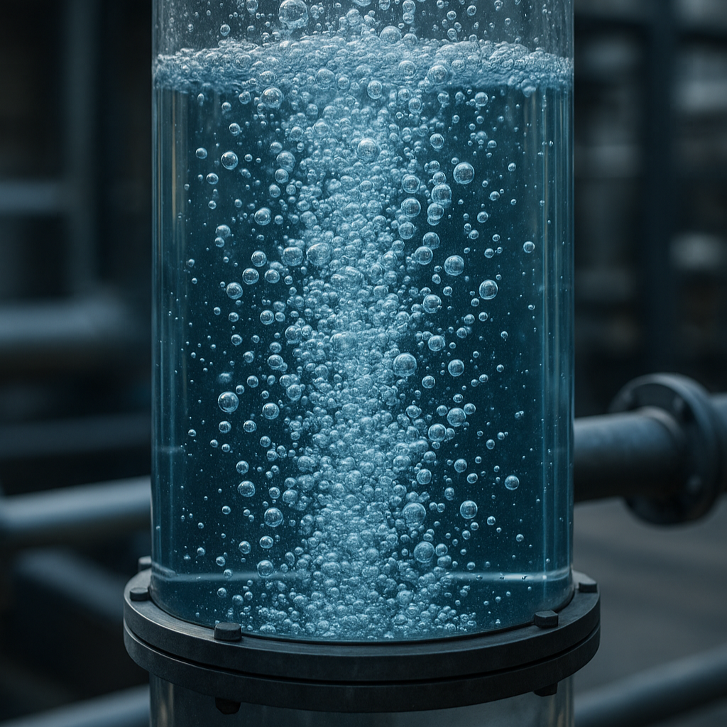
Examples: air bubbles in water, oil-water mixtures, sand in air (fluidized beds), boiling and condensation.
Key regimes:
Gas–liquid: bubbles, droplets, jets, boiling/condensation.
Liquid–solid: slurries, sedimentation, fluidized beds.
Gas–solid: pneumatic transport, cyclone separators, combustion with solid fuel.
Liquid–liquid: immiscible liquids, emulsions.
Why it matters: multiphase flows dominate many industrial systems, like reactors, heat exchangers, separators, combustion chambers, and spray systems.
Physical challenge: Each phase interacts by momentum, heat, and mass transfer across often complex interfaces.
2. Governing Equations and Intuition
Multiphase CFD models extend Navier–Stokes equations to more than one phase.
Volume fraction (α): fraction of control volume occupied by each phase.
Constraint: all α’s sum to 1.
Intuition: Think of each cell as a “box” partially filled with gas, liquid, solid fractions
Continuity equation (per phase): ensures mass conservation for each phase.
Momentum equation (per phase): Navier–Stokes with additional terms for interphase drag, lift, virtual mass, etc.
Intuition: describes how one phase pulls/pushes the other
Closure problem: requires empirical or semi-empirical interfacial exchange laws (drag, heat transfer correlations).
Limitation: accuracy depends on quality of these closures
3. Modeling Approaches in Fluent (with physical intuition)
Mixture Model
Treats phases as interpenetrating but solves one momentum equation for mixture + slip velocity equation.
Good for: bubbly, slurry, or dispersed flows where particles move differently but stay well mixed.
Advantage: cheaper than full Eulerian; handles up to moderate dispersed phase fractions.
Limitation: not great for sharp interfaces.
Volume of Fluid (VOF)
Tracks distinct interfaces between immiscible fluids.
Solves one set of equations, adds volume fraction transport for each phase.
Best for: free surface flows, sloshing, stratified layers, waves, filling/draining tanks.
Limitation: doesn’t resolve dispersed bubbles/droplets well.
Eulerian (Multi-fluid Model)
Solves full Navier–Stokes for each phase (Euler–Euler).
Most general, can model dense multiphase flows, fluidized beds, strong coupling.
Requires detailed closure models for drag, collisions, etc.
Computationally expensive.
Discrete Phase Model (DPM / DDPM)
Lagrangian tracking of individual particles as point masses.
Valid for low dispersed phase volume fraction:
DPM: <10%
DDPM: up to ~30%
Used in: sprays, fuel injection, particle trajectories.
Assumes rigid spherical particles, no deformation.
4. Strategy and Model Selection
Gas-liquid bubbly/slurry (>10% dispersed): Mixture or Eulerian.
Free surfaces/stratified/slug flow: VOF.
Particle-laden dilute (<10%): DPM.
Dense particle beds/fluidized reactors: Eulerian.
Pneumatic transport: Mixture (homogeneous) or Eulerian (granular).
5. Important Parameters
Dispersed phase volume fraction -> dilute vs. dense regime.
Dilute (<10^-3): negligible particle-particle interaction.
Dense (>10^-3): collisions, four-way coupling important.
Dispersed phase size: can be constant, user-defined correlation, interfacial area (Sauter mean), or from population balance model.
Mesh/time resolution: resolving individual bubbles/droplets directly is impractical in industry → use averaged models.
6. Industrial Applications
Gas–liquid: bubble columns, nuclear reactors, spray cooling, fire sprinklers.
Liquid–solid: slurry transport in mining, sewage treatment, filtration, hydro-transport.
Gas–solid: pneumatic transport, cyclones, coal combustion.
Liquid–liquid: emulsifiers, fuel cells, phase separators.
Rule of thumb: identify the dominant physical mechanism (interface, mixing, sedimentation, etc.) and choose model accordingly
Summary
Multiphase CFD is inherently complex, since real flows involve strong coupling between phases and often overlapping flow regimes. The key to effective modeling lies in choosing the right level of description: mixture models and DPM for simpler or dilute cases, Eulerian models for dense interactions, and VOF for sharp interfaces. Every approach involves assumptions and trade-offs: from neglecting particle deformation to relying on empirical drag correlations, but with a careful selection, robust and useful predictions can be achieved. In practice, the model should be matched to the dominant physics of interest, starting with simplified representations and refining as needed