

Turbomachinery 3: Equations and Principles
Understanding turbomachinery through CFD requires more than solving the Navier–Stokes equations. The motion of rotating blades changes how momentum, energy and pressure interact, while the numerical model must represent complex blade passages, periodic flow structures and near-wall effects. This chapter connects the governing physics of turbomachinery with the practical decisions involved in constructing reliable CFD models, from reference frames and rothalpy to mesh topology and numerical accuracy.

1. Introduction: From blade geometry to fluid mechanics
In Chapter 2, the focus was on the geometry of turbomachinery blades: how their profiles are defined, how blade angles vary along the span, and how geometric characteristics such as pitch, chord, camber and meridional length describe a blade row.
Geometry establishes the shape of the flow passage, but it does not tell us how the fluid will behave inside it.
A rotating compressor blade, for example, changes the direction and angular momentum of the incoming fluid while transferring mechanical energy into the flow. A turbine performs the reverse energy conversion, extracting energy from the fluid through the torque generated on its rotating blades.
Predicting these processes requires three interconnected descriptions:
Physical: Conservation of mass, momentum and energy, including the effects of rotation.
Mathematical: A suitable set of governing equations, modelling approximations and boundary conditions.
Numerical: A computational domain and mesh capable of representing the blade passage and resolving the relevant flow structures.
The central engineering challenge is choosing a description that is sufficiently accurate without making the calculation unnecessarily expensive.
2. Conservation equations in turbomachinery
2.1 The control-volume approach
The starting point is the conservation of mass, momentum and energy. These laws remain valid regardless of whether the fluid passes through a stationary duct, a rotating compressor or a turbine.
The integral formulation considers a finite control volume bounded by a control surface. Physical quantities can accumulate inside the volume, enter or leave through its boundaries, or change because of forces and energy transfer.
For a blade passage, this is particularly useful because the inlet and outlet flows can be related to the forces and torque acting on the blades.
The differential formulation describes the same conservation principles locally, at individual points in the flow field. It provides the basis for numerical methods that divide the domain into computational cells.
2.2 Conservation of mass
Mass conservation requires that any difference between the mass entering and leaving a control volume must correspond to mass accumulation inside it.
For steady flow with no mass sources, the total mass flow rate entering a blade passage equals the mass flow rate leaving it.
This does not mean that density or velocity must remain constant. In a compressor, the density may increase substantially while the passage area and velocity change. The mass flow rate remains consistent through the corresponding adjustments.
In CFD, mass imbalance is therefore one of the first quantities to check when evaluating a converged solution.
2.3 Conservation of momentum
Momentum conservation relates changes in fluid motion to the forces acting on it.
The principal contributions include pressure forces, viscous stresses and, where applicable, body forces. In turbomachinery, pressure forces on the blade surfaces are particularly important because they generate the aerodynamic loading responsible for torque and energy transfer.
The flow is inherently three-dimensional. Velocity can change in the axial, radial and circumferential directions, and blade curvature produces pressure gradients that redirect the fluid.
This is why a purely one-dimensional description can estimate overall performance but cannot fully represent blade loading, secondary flow or local losses.
2.4 Conservation of energy
The energy equation accounts for the transport and transformation of internal, kinetic and other relevant forms of energy.
In stationary passages, changes in kinetic energy and pressure are connected through the flow's energy balance. In rotating blade rows, mechanical work is also exchanged between the rotor and the fluid.
For an adiabatic stationary blade row without shaft work, stagnation enthalpy is conserved under the corresponding assumptions. For a rotating blade row, the appropriate conserved quantity under ideal steady conditions is instead rothalpy.
That distinction is fundamental to understanding turbomachinery CFD.
3. Absolute and rotating reference frames
3.1 Why reference frames matter
A stationary observer and an observer rotating with a compressor blade describe the same physical flow differently.
In the absolute reference frame, the blade moves through the fluid. In the relative reference frame, the blade is stationary, while the fluid velocity is measured relative to the blade motion.
This distinction is particularly useful because a flow that is unsteady from the stationary observer's perspective may be approximately steady relative to a rotating blade row.
For a rotor operating at constant rotational speed, a rotating reference frame can therefore simplify the numerical problem considerably.
The relationship between absolute and relative velocity is:
V = W + U
where:
V is the absolute fluid velocity.
W is the relative fluid velocity.
U is the local blade velocity, determined by angular velocity and radius.
Because blade speed increases with radius, the transformation between absolute and relative velocity varies along the blade span.
3.2 The velocity triangle
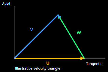
The velocity triangle is a geometric representation of the relationship between the three velocity vectors.
Its importance extends beyond coordinate transformations. Blade inlet and outlet angles, incidence, flow turning and angular momentum exchange all depend on the velocity components represented by these triangles.
For a rotor, the relative flow direction is particularly important because it determines how the fluid approaches and follows the blade surface.
3.3 Apparent forces in a rotating frame
When the conservation equations are expressed in a rotating reference frame, additional acceleration terms appear.
The two principal contributions for constant angular velocity are:
Centrifugal acceleration is associated with the rotation of the reference frame and depends on the distance from the rotational axis. It contributes to the radial momentum balance.
Coriolis acceleration arises when the fluid moves relative to the rotating reference frame. It depends on both the angular velocity and the relative fluid velocity.
These terms are not additional physical interactions introduced by the blades. They arise because the equations are being expressed in a non-inertial coordinate system.
In a rotating passage, the pressure field must balance the combined effects of fluid acceleration, curvature, rotation and viscous stresses. Consequently, the radial pressure distribution cannot generally be understood using axial flow considerations alone.
3.4 Axisymmetric coordinate systems
Turbomachinery geometry naturally suggests cylindrical coordinates, with axial, radial and circumferential directions.
For annular passages, the meridional plane provides a useful representation of the flow path from inlet to outlet, including changes in hub and casing radius.
An orthogonal axisymmetric coordinate system can be adapted to this geometry. This simplifies the description of certain flow components and geometric relationships, particularly when the machine has a smooth annular flow path.
However, an axisymmetric representation cannot reproduce all three-dimensional blade-passage phenomena. Individual blades introduce circumferential variations, and their loading produces flow structures that vary between the pressure and suction surfaces.
4. Angular momentum and energy transfer
4.1 Why angular momentum is central to turbomachinery
A turbomachine exchanges mechanical power through torque about its rotational axis.
Linear momentum conservation describes the forces acting on the fluid, but angular momentum conservation provides the most direct connection between blade forces and shaft torque.
The angular momentum carried by the fluid depends on its radius and circumferential velocity component.
For a steady blade row, the torque exerted on the fluid is related to the difference between the angular momentum transported through the inlet and outlet.
In simplified notation:
Torque = mass flow × change in (radius × tangential velocity)
This relationship explains why changing the circumferential component of velocity is essential to energy transfer.
A rotor can strongly redirect the flow without producing a corresponding shaft-work exchange if the relevant angular momentum change is zero.
4.2 Euler's turbomachinery equation
The Euler turbomachinery equation connects shaft work with the change in fluid angular momentum.
For a rotor, the specific work transferred to the fluid can be written conceptually as:
Specific work = U₂ × Vθ₂ − U₁ × Vθ₁
Here, U represents blade speed and Vθ the tangential component of absolute velocity. Subscripts 1 and 2 refer to the inlet and outlet.
With this sign convention, positive work corresponds to energy transferred from the rotor to the fluid, as in a compressor. A turbine normally produces a negative value because the fluid transfers energy to the rotor.
This relationship has an important engineering consequence: blade geometry influences energy transfer primarily through its effect on the velocity field and flow turning.
A compressor blade must guide the fluid so that its angular momentum increases in the intended manner. A turbine blade must generate the appropriate reduction in fluid angular momentum to produce useful torque.
The actual process is more complicated than an ideal velocity-triangle calculation because viscous effects, secondary flows and losses influence the exit velocity distribution.
4.3 Torque, rotational speed and power
Mechanical power is related to torque and angular velocity:
Power = Torque × angular velocity
At a fixed angular velocity, increasing torque increases the power exchanged between the rotor and the fluid.
Combining this relationship with angular momentum conservation gives a direct connection between the measured flow field and the mechanical performance of a turbomachine.
This is particularly valuable in CFD because shaft torque and power can be evaluated from aerodynamic forces or from angular momentum fluxes, subject to consistent definitions and accounting for relevant contributions.
5. Rothalpy and energy conservation in rotating machinery
5.1 Why stagnation enthalpy alone is insufficient
In a stationary, adiabatic passage without work transfer, stagnation enthalpy is conserved for steady flow under the usual ideal assumptions.
A rotating passage behaves differently. The blades exchange mechanical work with the fluid, so stagnation enthalpy can change between inlet and outlet.
A different energy quantity becomes particularly useful when the flow is described relative to the rotating blade row.
This quantity is called rothalpy.
5.2 Physical meaning of rothalpy
Rothalpy combines the fluid's thermodynamic state and kinetic energy with the effects associated with rotation.
It can be expressed in either of two equivalent forms:
I = h₀ − U × Vθ
or
I = h + W²/2 − U²/2
where h₀ is stagnation enthalpy, h is static enthalpy, and the remaining terms describe absolute tangential motion, relative kinetic energy and blade speed.
Rothalpy is particularly important because it remains constant along streamlines in a steady, adiabatic and inviscid rotating flow.
This provides a useful counterpart to stagnation enthalpy conservation in stationary passages.
5.3 Engineering interpretation
Consider a compressor rotor.
As the fluid travels through the rotor, the blade performs work on it. Its stagnation enthalpy therefore increases.
However, the quantity U × Vθ also changes. Under ideal steady conditions, these changes balance so that rothalpy remains constant along a streamline.
In a turbine, the direction of energy transfer is reversed, but the same conservation principle applies.
The significance is that the energy balance can be interpreted consistently within the rotating frame without treating every change in stagnation enthalpy as an unexplained energy source.
5.4 Entropy and irreversibility
Rothalpy conservation depends on assumptions that are not perfectly satisfied in real machines.
Viscous stresses, heat transfer and irreversible flow processes modify the energy balance. Entropy generation provides an important measure of these irreversible effects.
In an approximately adiabatic turbomachine, entropy increases are closely associated with mechanical energy dissipation.
This is why a CFD simulation should not be assessed only by its predicted pressure rise or torque. The distribution of entropy and other loss-related quantities can help identify regions where the machine's aerodynamic performance deteriorates.
Typical areas of interest include blade boundary layers, wakes and regions of strong velocity gradients.
6. Levels of approximation in turbomachinery CFD
The full governing equations contain more physical information than is practical to resolve in every engineering simulation.
The appropriate mathematical model depends on the flow phenomena of interest, the available computational resources and the required accuracy.
6.1 Hierarchy of flow models
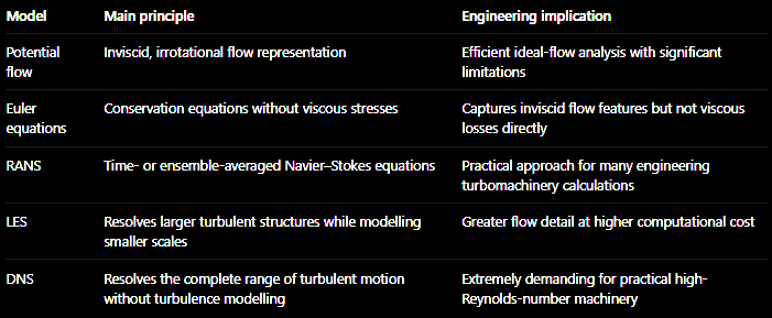
These descriptions form a progression in physical resolution and computational requirements, although each involves different assumptions and is appropriate for different applications.
6.2 Direct Numerical Simulation
DNS solves the unsteady Navier–Stokes equations without introducing a turbulence model.
The difficulty is that turbulent flow contains a wide range of spatial and temporal scales. At high Reynolds numbers, the smallest relevant structures become much smaller than the characteristic dimensions of the machine.
Resolving them requires a rapidly increasing number of computational cells and time steps.
The computational effort consequently grows very strongly with Reynolds number. For the Reynolds numbers encountered in industrial turbomachinery, DNS is generally not a practical method for routine full-machine calculations.
Its main value lies in highly resolved studies that improve understanding of fundamental turbulent-flow behaviour.
6.3 Large Eddy Simulation
LES reduces the computational burden by resolving the larger turbulent structures and modelling the effects of smaller unresolved scales.
This is especially relevant when large-scale unsteady flow structures strongly influence the behaviour of the machine.
However, the need to resolve substantial turbulent motion in both space and time makes LES considerably more expensive than conventional RANS calculations, especially near solid walls.
6.4 Reynolds-Averaged Navier–Stokes equations
RANS introduces a statistical description of turbulent flow.
Rather than directly resolving every turbulent fluctuation, the governing equations describe averaged quantities. The influence of turbulent fluctuations introduces additional terms that must be represented through a turbulence model.
This provides a practical compromise between physical detail and computational cost.
For many turbomachinery engineering problems, RANS is a suitable starting point because it can predict the main flow structure and performance characteristics without resolving the full turbulent spectrum.
Nevertheless, its accuracy depends on the selected turbulence closure and the nature of the flow being simulated. Strong separation, highly unsteady structures and complex interactions can introduce significant modelling uncertainty.
6.5 Euler and potential-flow approaches
Removing viscous stresses leads to the Euler equations.
These retain the effects of pressure, inertia and compressibility but do not directly represent viscous boundary layers or viscous dissipation.
Potential-flow formulations introduce further simplifications by assuming irrotational motion, with additional assumptions depending on the formulation.
Such methods can be useful when the principal objective is to understand ideal flow turning and pressure distributions rather than accurately resolve viscous losses.
The important limitation is that removing viscous physics also removes mechanisms that strongly influence real turbomachinery performance.
7. Initial and boundary conditions
The governing equations do not uniquely determine the flow unless appropriate initial and boundary conditions are supplied.
In turbomachinery, boundary-condition selection requires particular care because the flow may be compressible, rotational, periodic and influenced by neighbouring blade rows.
7.1 Inlet and outlet conditions
At an inlet, the numerical model must provide sufficient information to describe the incoming flow. Depending on the mathematical formulation and flow regime, this may involve pressure, temperature, velocity components or flow direction.
At the outlet, the admissible conditions depend on the propagation of information through the flow.
For subsonic compressible flow, disturbances can propagate both upstream and downstream. The boundary conditions must therefore respect the characteristics of the governing equations.
For supersonic flow, the propagation of information is more restricted, changing which variables can be imposed independently.
Over-specifying a boundary can create an inconsistent mathematical problem, while under-specifying it leaves the solution insufficiently constrained.
7.2 Solid walls
Blade, hub and casing surfaces impose constraints on the fluid motion.
For viscous flow, the no-slip condition represents the interaction between the fluid and the solid surface. On stationary walls, the fluid velocity at the wall is zero in the corresponding stationary frame.
On rotating walls, the wall velocity must be consistent with the frame of reference.
For inviscid formulations, the primary wall constraint is impermeability: fluid cannot pass through the solid surface, but tangential slip is permitted.
The distinction matters because inviscid and viscous calculations represent different physical mechanisms.
7.3 Periodicity conditions
A turbomachine contains many geometrically repeated blade passages. Simulating the entire circumference is often unnecessary when the flow is assumed to repeat periodically.
A single blade passage can then be modelled with periodic boundaries connecting its two circumferential sides.
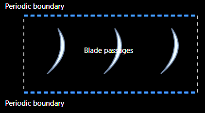
Conceptual unwrapped blade-row view. The two periodic boundaries represent corresponding locations in neighbouring passages.
Periodicity may be spatial or temporal.
Spatial periodicity represents repetition around the circumference. Temporal periodicity describes repetition over time, which becomes important for certain unsteady rotor–stator interactions.
Numerically, periodic boundaries may be implemented through suitable cell connectivity or ghost-cell procedures.
The assumption of passage periodicity is powerful, but it must be physically justified. A single-passage model cannot represent circumferential disturbances that do not repeat over the chosen sector.
7.4 The Kutta condition
For lifting aerodynamic profiles with a sharp trailing edge, the inviscid flow solution may require an additional condition to determine circulation.
The Kutta condition selects a physically meaningful flow behaviour at the trailing edge, avoiding the singular velocities that can otherwise arise in idealized inviscid formulations.
In numerical Euler calculations, the condition is often not imposed explicitly. Numerical dissipation can produce a solution with finite trailing-edge velocities and appropriate circulation.
This is an important example of how mathematical idealizations and numerical methods interact.
7.5 Boundary-layer displacement and transpiration
Inviscid calculations do not directly resolve viscous boundary layers. Nevertheless, boundary-layer development changes the effective flow area available to the external flow.
One approximation is to modify the computational boundary using the boundary-layer displacement thickness.
Another approach modifies the wall-normal velocity condition, allowing a transpiration representation.
These techniques introduce selected effects of the boundary layer without solving the full viscous flow field.
Their usefulness depends on the required accuracy and the validity of the approximations.
8. From governing equations to the computational mesh
A numerical solver requires the continuous fluid domain to be divided into a finite collection of computational cells.
For turbomachinery, this process is challenging because blade passages combine several geometrically demanding features:
Curved pressure and suction surfaces.
Narrow leading-edge and trailing-edge regions.
Hub and shroud boundaries.
Strong spanwise changes in geometry.
Periodic circumferential boundaries.
Possible blade-tip or hub-tip clearances.
The mesh must follow these geometric features while maintaining acceptable cell quality.
An unsuitable mesh can introduce numerical errors even when the governing equations and physical models are correctly selected.
8.1 Why structured meshing is attractive
Structured meshes use an organized arrangement of computational cells, with predictable connectivity between neighbouring elements.
This is particularly useful in blade passages because the geometry has a recognizable flow direction and repeated structure.
A structured mesh can align cells with important geometric boundaries and provide controlled refinement near blade surfaces.
However, creating a high-quality structured mesh around a three-dimensional blade requires more than simply distributing points uniformly through the passage.
The arrangement of blocks and their connectivity must be designed to accommodate the blade geometry.
This arrangement is called the mesh topology.
9. Geometry preparation in ANSYS TurboGrid
TurboGrid is designed specifically for generating turbomachinery blade-passage meshes.
It can operate as a standalone application or within ANSYS Workbench. The Workbench environment is especially useful when the mesh is part of a connected design and simulation workflow.
A typical workflow is:
BladeGen / Geometry → TurboGrid → Fluent / CFX
Geometry definition → topology and mesh → flow solution
When geometry changes, the connected project can update the downstream mesh and simulation components.
This is valuable for design comparisons, mesh sensitivity studies and parameterized blade investigations.
9.1 Importing the blade geometry
The geometric description must identify the blade surfaces, hub, shroud and relevant flow boundaries.
TurboGrid supports different geometry input procedures, allowing the blade passage to be reconstructed from suitable geometric data.
The important requirement is not simply that the imported geometry looks correct. It must also contain sufficient information to generate the blade and passage surfaces consistently.
9.2 Blade-surface reconstruction
A blade surface can be constructed through a two-stage procedure.
First, curves are generated from the available geometric points. Second, the curves are connected to create a continuous surface through a process called lofting.
Two principal lofting directions are available:
Spanwise lofting uses blade-profile curves and connects them along the blade span.
Streamwise lofting uses curves formed by connecting corresponding points on adjacent blade profiles.
For streamwise lofting, the profiles must have compatible point counts, ordering and correspondence. Otherwise, the resulting surface may be distorted.
9.3 Curve and surface representations
TurboGrid supports piecewise-linear and B-spline curve representations.
Piecewise-linear curves connect points using straight segments. B-splines construct smoother interpolated curves, which can be useful when relatively few points describe a profile.
For surface construction, ruled surfaces connect neighbouring curves using linear paths, while B-spline surfaces use curved interpolation.
The predefined geometry methods include:

The choice affects how the supplied blade coordinates are converted into the surface used for meshing.
9.4 Hub, shroud and tip clearances
By default, TurboGrid assumes the blade extends between the hub and shroud.
For a blade with a clearance at one end, the corresponding tip geometry must be defined.
TurboGrid provides clearance-definition options such as constant span, normal distance, variable normal distance and profile-based definitions.
This is important because a tip clearance creates an additional flow region between the blade and the adjacent stationary or rotating surface.
The geometry and mesh must represent this gap if its flow behaviour is part of the simulation objective.
9.5 Periodic boundaries and interfaces
Periodic boundaries identify corresponding circumferential surfaces of a repeated blade passage.
TurboGrid allows the location of these surfaces to be adjusted using a blade-bias factor. This can prevent the periodic boundary from passing too close to, or intersecting, the blade surface.
For multistage configurations, the inlet or outlet interface can also be adjusted with reference to adjacent blade-row geometry.
The goal is to construct compatible computational domains for the different rows before connecting them in the flow solver.
10. Mesh topology and automatic topology generation
Mesh topology defines how the computational blocks are arranged and connected around the blade.
This is different from mesh density. Increasing the number of elements refines an existing mesh, whereas changing topology modifies the underlying arrangement of computational regions.
10.1 H-grid and O-grid concepts
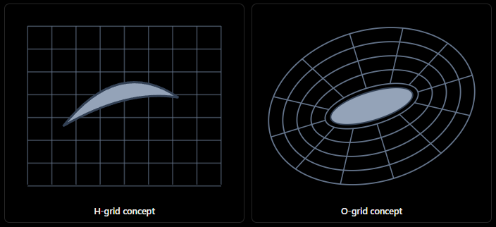
Conceptual illustrations of grid arrangements. Actual TurboGrid topology is adapted to blade and passage geometry.
An H-grid uses a structured arrangement extending through a region, while an O-grid wraps around a geometric feature such as a blade.
The O-grid arrangement is especially useful for controlling mesh refinement around blade surfaces, including the boundary-layer region.
10.2 Automatic Topology and Meshing (ATM)
TurboGrid includes an automatic topology and meshing approach known as ATM.
Rather than relying on a single smoothing operation, ATM combines several processes:
Automatic topology generation.
Placement of topology around the geometry.
Background mesh generation.
Mesh sizing.
Mesh generation and smoothing.
The aim is to generate a suitable topology with relatively limited manual intervention.
An important feature is that topology positioning can be independent of the selected mesh size. This allows mesh density to be changed without necessarily redesigning the underlying block arrangement.
ATM also supports O-grid refinement control while maintaining the overall topology.
This makes it particularly useful for systematic mesh studies, where different resolutions should be compared without introducing unnecessary changes in mesh structure.
11. Mesh sizing and refinement
A computational mesh must balance resolution and computational expense.
Adding elements everywhere increases the total cell count, but not every region requires the same spatial resolution.
TurboGrid therefore provides several mesh-sizing controls.
11.1 Global mesh sizing
Global sizing establishes the approximate overall resolution of the blade passage.
It is a convenient starting point, but it should not be the only mesh control used for a demanding CFD simulation.
A global increase in resolution may be computationally expensive while failing to target the most important local flow regions efficiently.
11.2 Passage and spanwise sizing
The passage mesh can be controlled in the spanwise direction, from hub to shroud.
Available distribution approaches include proportional spacing, specified element count and size, boundary-layer-oriented distributions, and uniform spacing.
Uniform spacing maintains approximately constant element dimensions along the span. Nonuniform distributions allow additional resolution near selected locations.
The appropriate distribution depends on the blade geometry and the regions where flow gradients are expected.
11.3 Boundary-layer refinement
Near a solid surface, viscous effects produce steep velocity gradients.
The mesh must therefore provide suitable resolution normal to the blade surface if the numerical model is intended to resolve these gradients.
TurboGrid provides boundary-layer refinement controls associated with the O-grid region.
The important point is that boundary-layer refinement is not simply a matter of increasing the total element count. The distribution and progression of element sizes near the surface also matter.
11.4 Tip-gap mesh sizing
A blade-tip clearance can be much smaller than the overall passage dimensions.
If the gap is represented with insufficient resolution, important variations in velocity and pressure may not be captured adequately.
TurboGrid provides separate controls for hub-tip and shroud-tip regions so that these areas can be refined without applying the same resolution throughout the entire domain.
11.5 Inlet and outlet domains
The mesh must also extend upstream and downstream of the blade.
These regions provide space for the inlet and outlet boundary conditions and for the development of the flow entering or leaving the blade passage.
TurboGrid supports H-grid approaches for inlet and outlet domains, including meshing in parametric space. The number of elements in the meridional direction can be adjusted independently.
11.6 Mesh layers
A three-dimensional blade-passage mesh can be examined through individual spanwise layers.
This is useful because mesh quality may vary significantly between the hub, midspan and shroud.
A mesh that looks acceptable at midspan may contain highly distorted elements near an endwall or tip-clearance region.
Inspecting individual layers helps identify these localized problems before the mesh is transferred to the CFD solver.
12. Mesh quality and optimization
Generating a mesh is not the final step. The mesh must be assessed to determine whether its elements are geometrically suitable for numerical calculations.
TurboGrid provides several quality measures.
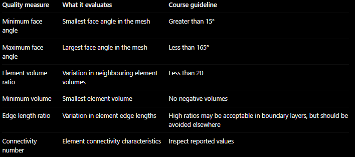
These values are mesh-quality guidelines, not a guarantee of solution accuracy.
12.1 Face angles
Highly distorted cell faces can reduce numerical accuracy and affect solver robustness.
Very small or very large face angles indicate that an element deviates substantially from the desired geometric arrangement.
The mesh should therefore avoid excessive angular distortion, particularly in regions where important flow gradients occur.
12.2 Element volume ratio
A large difference between neighbouring cell volumes can create abrupt changes in spatial resolution.
Such changes may adversely affect numerical discretization and convergence.
The element volume ratio provides a way to identify these transitions.
12.3 Edge length ratio
The edge length ratio characterizes the difference between element dimensions.
High aspect ratios are not automatically unacceptable. Boundary-layer meshes intentionally use thin elements in the wall-normal direction and longer dimensions along the surface.
The distinction is whether the anisotropy is purposeful and aligned with the physical problem.
Away from boundary layers, unnecessarily large edge length ratios should generally be avoided.
12.4 Negative volumes
A negative cell volume indicates an invalid element orientation or geometric configuration.
Such elements must be corrected before proceeding to the solver.
12.5 Improving mesh quality
When quality requirements are not satisfied, several adjustments are available:
Modify geometry definitions or inlet/outlet control curves.
Adjust global and boundary-layer sizing.
Change the spanwise distribution.
Add or modify mesh layers.
Introduce edge splits or adjust element counts.
A sensible approach is to identify the location and nature of the problematic elements before modifying the mesh.
Changing several settings simultaneously may improve the reported statistics, but it makes it difficult to determine which modification was responsible.
13. Mesh sensitivity and parameterization
Even a mesh that satisfies geometric quality requirements may not provide a sufficiently accurate numerical solution.
The predicted flow field can still depend on mesh resolution.
A mesh sensitivity study investigates how the quantities of interest change when the computational mesh is refined.
For turbomachinery, these quantities may include pressure ratio, mass flow, torque, power and aerodynamic losses.
The principle is to compare multiple mesh resolutions while maintaining consistent geometry, physical models and boundary conditions.
If the relevant output quantities change only slightly with further refinement, the numerical solution becomes less sensitive to mesh resolution.
This does not eliminate modelling uncertainty, but it helps separate discretization effects from other sources of error.
13.1 Parameterization in Workbench
TurboGrid can expose selected input values as Workbench parameters.
This allows the same project structure to be used for different mesh settings or blade geometries.
For example, a mesh sensitivity study can be organized around several target mesh sizes while maintaining a consistent downstream CFD workflow.
13.2 State files, session files and batch operation
TurboGrid also supports saving application states and recording sequences of operations.
Session files and batch execution are useful for automating repeated meshing tasks.
These capabilities are especially valuable when performing parameterized blade studies or generating multiple meshes for comparison.
However, automation does not eliminate the need to inspect the resulting geometry and mesh quality. A successfully completed batch operation does not necessarily imply that the mesh is suitable for the intended simulation.
14. Connecting the physics and numerical model
The governing equations and mesh-generation procedures are not independent topics.
They describe different parts of the same modelling problem.
The conservation equations establish which physical quantities must be represented. The chosen approximation determines which flow phenomena can be predicted. The geometry and mesh determine how accurately the selected equations can be discretized in the blade passage.
Consider a compressor rotor.
The angular momentum equation connects the change in tangential velocity to rotor torque. The energy equation connects this torque to work transfer, while rothalpy provides an appropriate energy description in the rotating frame.
To predict these quantities numerically, the model must represent the blade shape and flow passage. The mesh must capture the relevant pressure and velocity distributions, while the boundary conditions must be consistent with the physical operating conditions.
A poorly constructed mesh may produce inaccurate blade loading even when the mathematical model is appropriate.
Conversely, an exceptionally fine mesh cannot recover physical mechanisms excluded by the governing equations or modelling assumptions.
This leads to an important distinction:
Numerical resolution determines how accurately the chosen mathematical model is solved; physical modelling determines which phenomena the model can represent.
Both must be considered when evaluating a CFD result.
15. Practical CFD workflow
A useful turbomachinery CFD workflow can be organized into six stages.
Define the physical problem
Identify the machine type, operating conditions, relevant blade rows, rotational speeds and required performance quantities.
Select the mathematical model
Choose the governing-equation approximation, reference frame, flow assumptions and boundary conditions.
Prepare the blade-passage geometry
Import or reconstruct blade surfaces, hub and shroud boundaries, periodic surfaces and any necessary clearances.
Generate the mesh
Establish topology, global and local sizing, boundary-layer refinement and spanwise distributions.
Evaluate mesh quality and numerical sensitivity
Check element-quality measures, investigate problematic regions and compare multiple mesh resolutions when necessary.
Solve and evaluate performance
Examine convergence, conservation balances, pressure and velocity distributions, torque, work transfer and losses.
The workflow is iterative. Unexpected CFD results may reveal problems with the boundary conditions, geometry representation, mesh resolution or modelling assumptions.
A reliable simulation therefore requires more than achieving numerical convergence. The final solution must also be physically consistent and sufficiently insensitive to the numerical choices that should not dominate the engineering conclusions.
16. Final perspective
Turbomachinery CFD combines fundamental fluid mechanics with numerical approximations adapted to rotating blade passages.
Angular momentum conservation provides the connection between fluid turning and shaft torque. The Euler turbomachinery equation translates this relationship into energy transfer, while rothalpy provides a particularly useful description of energy conservation in rotating reference frames.
The governing equations can be solved at different levels of approximation, from inviscid descriptions to fully resolved turbulent simulations. Choosing between them involves balancing physical detail, computational expense and the objectives of the analysis.
The numerical mesh is equally important. TurboGrid provides specialized tools for reconstructing blade geometry, generating structured topology, controlling local refinement and evaluating mesh quality.
Ultimately, a credible turbomachinery simulation requires consistency between the physical assumptions, governing equations, geometry, mesh, boundary conditions and numerical solution.
A well-resolved mesh cannot compensate for an inappropriate physical model, and an advanced physical model cannot compensate for an inadequate computational domain.